
Improving Dataflow Pipelines for Text Data Processing
This post discusses recipes to improve Cloud Dataflow pipelines for large-scale datasets involving sequential text data.


Data scale is crucial at Carted. The machine learning (ML) capabilities we're building need internet-scale data to power them. With such large-scale data regimes comes an obvious challenge of careful engineering that allows us to handle these regimes effectively and efficiently. To do this, we leverage several managed services from Google Cloud, such as Dataflow, BigQuery, and others.
In this article, we'll share a few recipes to improve Dataflow pipelines when dealing with sequence data. These methods came from our experience of processing and preparing large datasets for ML use. We hope you’ll apply these recipes to your own Dataflow pipelines to improve their performance.
Code
The techniques discussed in this post are implemented within a demo pipeline, which can be run using Cloud Dataflow:
 carted
About the data
The raw data available to us are text descriptions of products available on ecommerce websites. Each description comprises one or more sentences extracted as individual sentences, thus generating multiple text sequences per datum.
Our data processing setup
The product descriptions are stored in a BigQuery table, and we process this data with an Apache Beam pipeline run on Dataflow. If you want to get a quick overview of the two, this resource is a good place to start. We encode the text features using a conditional BERT model that includes tokenization and computing the text embeddings with the pre-trained BERT model. For this part, we use TensorFlow Hub. We define all the different preprocessing steps as a part of an Apache Beam pipeline.
We break the data processing pipeline into three concrete Beam steps:
- Reading the descriptions from BigQuery.
- Tokenizing and encoding the sentences per description followed by a pooling operation. The pooling operation typically involves taking the mean or the max per dimension of the sentence vectors of a description to obtain a single vector for the whole description.
- Writing the vectors to a Google Cloud Storage (GCS) bucket in a serialized format, namely TensorFlow Records.
Optimizing our pipeline
To reduce compute waste, several optimizations can be made on the pipeline described above—mostly to step two. The optimizations were performed keeping certain factors in mind:
- The optimizations should be simple enough to implement in a short timeframe. Even if there is room for improvement, development time plays a crucial role.
- GPUs can be leveraged to accelerate the computations for the embeddings of the tokenized text features. But GPUs are expensive, and hence it was decided not to use them for our purpose. But in general, the optimizations should also lead to improvement in performance on GPUs if they are to be used in the future.
- To track the performance of the pipeline, only the wall time of the relevant steps were monitored to avoid accounting for the time taken for setup and teardown of the Dataflow job. Note that wall time is different from the total pipeline time reported by the Dataflow UI.
Listed below are the various optimizations that were applied to the existing pipeline. Ideally, these techniques should apply to any scenario where text data needs to be processed in a similar way. We first describe the motivations behind each optimization and then go into the full details.
Batches with variable sequence lengths
The sentence encoder model expects the tokenized text features to have a uniform length of no more than 512 tokens, with a default length of 128. So, we have two options:
- We maintain a global sequence length of 512. That is, we pad all sequences with tokens less than 512 with a default padding token till they have 512 tokens in total. We do this to make the most of our data and the sentence encoder while keeping the code simple. This approach is depicted in Figure 1.
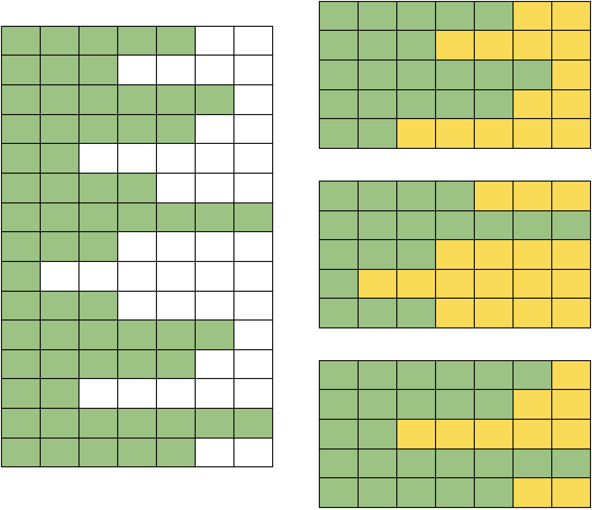
- We first derive the maximum sequence length for a given batch of sequences and do the rest of the processing with the derived sequence length for the corresponding batch. This approach is depicted in Figure 2.
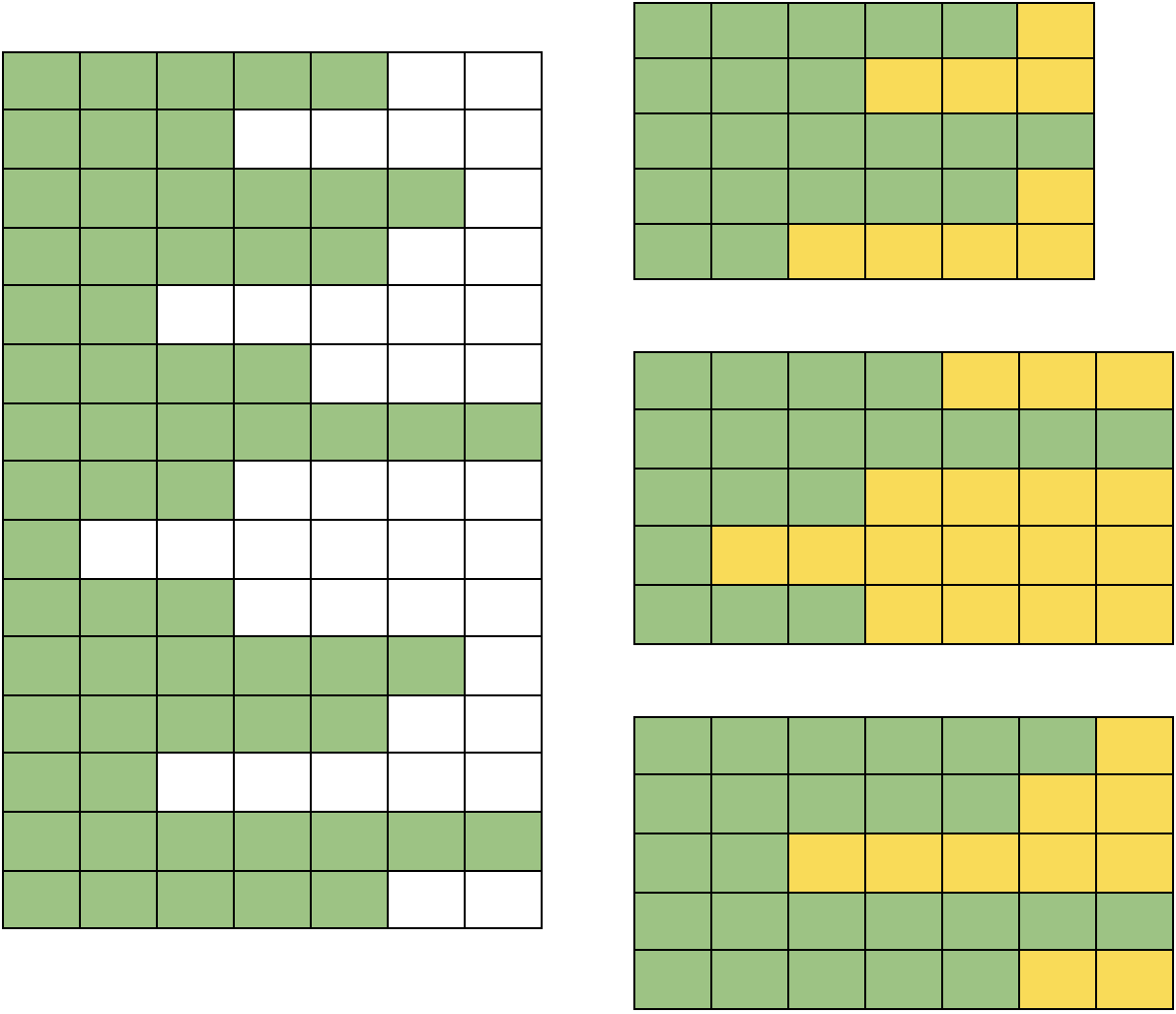
In our pipeline, we implemented the second option because the first one can lead to a lot of compute waste as many batches may have much shorter sequence lengths than 512 and hence the sentence encoder will needlessly process a lot of padding tokens. For batches having a maximum sequence length of 512 or above, we truncate the sequences till the first 512 tokens. The implementation of this recipe was non-trivial and we intend to cover our approach in a future article.
Sorting before batching
In our unoptimized pipeline, once the description sentences of an example are tokenized, they are grouped into batches and these batches are encoded one after another. The encoder expects the sequences in a batch to be of the same length. Since all sentences are not necessarily of the same length, it’s common practice to use a predefined padding token. Padding is applied to all the sequences that are shorter than the longest sequence in the batch. This results in a batch with all sequences having the same length. While this technique works, it still leads to a lot of wasted compute since the padding tokens are processed by the BERT encoder (their contributions to the final output are masked). The compute waste is more severe when the average difference between the maximum sequence length and the length of all other sequences increases in a batch.
We grouped sequences of the same or similar length before batching in an attempt to save compute waste. We accomplished this by:
- Sort the tokenized description sentences and store them in a list called
sorted_sentences. - Encode non-overlapping, consecutive chunks from
sorted_sentences. - Unsort the resultant embeddings from step 2 to preserve the original order.
This process of sorting and unsorting for a given chunk_size looks like so in code:
# `tf` is aliased as `import tensorflow as tf`
# Encode with BERT in a batch-wise manner to prevent OOM.
len_idx = len(all_text_token_lens)
all_bert_encodings = []

# Sort sequences to reduce compute waste.
sort_idx = tf.argsort(all_text_token_lens, direction="DESCENDING", axis=0)
unsort_idx = tf.argsort(
    sort_idx, direction="ASCENDING", axis=0
)  # indices to unsort the sorted embeddings

sorted_all_text_tokens = tf.gather(all_text_tokens, sort_idx, axis=0)
sorted_all_text_token_lens = tf.gather(all_text_token_lens, sort_idx, axis=0)

for idx in range(0, len_idx, chunk_size):
    bert_encodings = compute_text_encoding(
        sorted_all_text_tokens[idx : idx + chunk_size],
        sorted_all_text_token_lens[idx : idx + chunk_size],
    )
    all_bert_encodings.append(bert_encodings)

all_bert_encodings = tf.concat(all_bert_encodings, axis=0)

# Unsort the encodings.
all_bert_encodings = tf.gather(all_bert_encodings, unsort_idx, axis=0)
One concept that becomes apparent after considering the optimization above is the concept of uniform batches. Formally, the uniformity of a batch can be defined as:
We now can say that the compute waste due to the processing of padding tokens per batch is inversely proportional to the uniformity of a batch. Figure 3 visually presents this approach of sorting a block of sequences with respect to their sequence lengths and then applying padding with the approach discussed earlier.
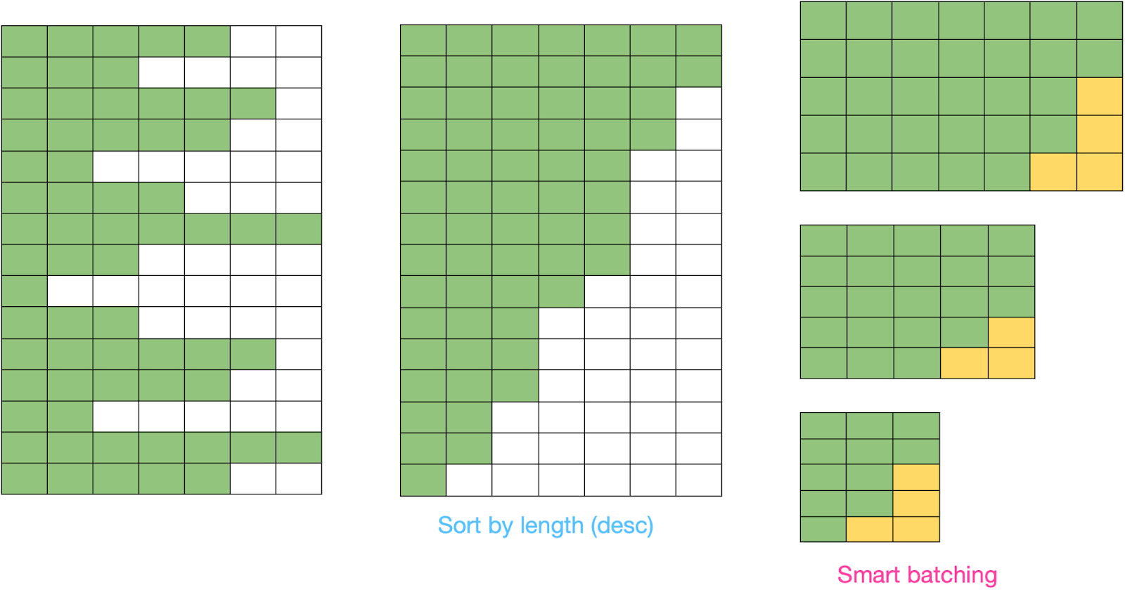
The reason for sorting the sequences in descending order is that if the chosen batch size is too large to fit in memory, we would get an out-of-memory (OOM) error at the very first batch. This allows us to reduce the batch size accordingly.
If the sequences were sorted in ascending order, we would have to wait for a decent amount of batches to be encoded before the sequence lengths of the batches increase enough to cause the OOM error (the worst case being the last batch throwing an OOM error) which might lead to hours of wasted compute.
In a way, sorting in a non-decreasing/descending order also makes the behavior of the inference process more predictable. If the first batch doesn't throw an OOM error, none of the subsequent batches will.
However, batching over unsorted data might lead to an OOM error at any time during the encoding process, and batching over data sorted in ascending order might lead to OOM error at the very end of the computation.
Decoupling tokenization and encoding
Tokenizing sentences for BERT is done via the BERT Tokenizer algorithm, a fairly CPU-bound process. Since there are not many numerical computations involved, this step cannot be sped up by using hardware accelerators or by special CPU instructions (such as the AVX instructions for Intel CPUs) for vector operations.
Encoding the tokenized sentences involves passing the (sorted) tokenized sequence of batches to the BERT model, which can be sped up significantly via hardware accelerators or vector instructions.
If we process sentences per example, we first have to:
- Tokenize all the sentences.
- Sort them according to the number of tokens per sentence.
- Perform batching and padding.
- Compute embeddings from the padded batches.
- Unsort the embeddings.
While this sounds reasonable, you’ll notice that once the accelerator has finished computing all the batches from a single example, it has to wait for the next example’s sentences to be processed from steps 1 to 4. This wastes precious time which adds up with every single example.
A much more streamlined way of doing this is to first tokenize all the examples at one go in one Beam step and then perform the encoding in the next Beam step. However, instead of encoding on a per-example basis, we could perform the encoding on a list of tokenized sentences collected across all the examples to minimize wait time for the accelerator. This is how it would look:
Substep 1:
- Tokenize the sentences for each example.
Substep 2:
- Collect the tokenized sentences from each example in a single list.
- Sort this list according to the number of tokens per sentence.
- Perform batching and padding.
- Compute embeddings from the padded batches.
- Unsort the embeddings.
Now, taking a closer look at substep 2, you’ll notice that the wait time for the accelerator is much shorter since it doesn’t need to wait for the tokenization to complete for the next example.
Another key advantage of this two-step process is that while sorting, a larger pool of sentences is available, leading to more uniform batches and even less compute waste.
The issue with the decoupling process above is that step 1 of substep 2 can easily lead to OOM errors when the total number of sentences is very large. Therefore, we feed the data to substep 2 in batches of tokenized sentences (not to be confused with the batching of tokenized sentences done inside substep 2) using Apache Beam’s BatchElements transform. This ensures that OOMs are avoided, but at the same time, a large number of sentences are grouped to make the most of the sorting process.
Another advantage of using Apache Beam’s BatchElements transform is that it intelligently figures out the optimal batch size between two given limits. If the batch size is too large, it might cause the workers to use swap memory which would degrade performance due to disk I/O. If the batch size is too small, then the encoding step needs to wait, which again degrades the performance of the whole pipeline. The BatchElements transform automatically analyzes the performance of the downstream steps (hence intelligent) to figure out the optimal batch size.
The final steps look like the following:
Substep 1:
- Tokenize the sentences for each example.
Substep 2:
- Batch the examples.
Substep 3:
- Collect the tokenized sentences from each example in the batch in a single list.
- Sort this list according to the number of tokens per sentence.
- Perform batching and padding.
- Compute embeddings from the padded batches.
- Unsort the embeddings.
This is a brief example implemented as an Apache Beam pipeline:
tfrecords = (
    p
    | "Read rows from BigQuery"
    >> beam.io.ReadFromBigQuery(
        query=query,
        use_standard_sql=True,
    )
    | "Tokenize text description"
    >> beam.ParDo(
        tokenize_descriptions,
        config=preprocessor_config,
    )
    | "Intelligently batch examples"
    >> beam.BatchElements(
        min_batch_size=5, max_batch_size=1000
    )
    | "Embed the text features"
    >> beam.ParDo(embed_examples)
    ...
Results
Now that we’ve discussed the key areas of improvement in our pipeline, it’s time to see the results. For a fair comparison, we used the same hardware infrastructure while running our experiments with and without the recipes we discussed.
We limited the number of maximum workers to 500 for Dataflow and used the n1-custom-1-8192-ext machine type for running our experiments. For each experiment, we started with a total of 21328 entries coming from BigQuery. We then generated a total of 1317247 data points from them (with tokenize_description()). In this case, each experiment corresponds to a Dataflow job.
| Experiment | Wall Time (lower is better) |
|---|---|
| Unoptimized pipeline | 3d 11h 0m 40s |
| Decoupled tokenization and encoding | 3d 5h 35m 39s |
| Sorting before batching + Batches with variable sequence lengths | 4h 14m 34s |
| Sorting before batching + Batches with variable sequence lengths + Decoupling tokenization and encoding | 2h 36m 46s |
From the above table, the impact of our optimizations is quite evident. Rather than taking more than three days, our pipeline now takes under three hours. We have also applied these optimizations to a much larger data regime to confirm their effectiveness.
We can further improve the overall performance of our pipeline by using a smaller encoder model but that may come at the expense of reduced end performance. We can even perform knowledge distillation to obtain a smaller model without compromising performance.
Conclusion
In this article, we shared three recipes to improve the performance of our text preprocessing pipeline, summarized as:
- Using batch-wise maximum sequence length for padding as opposed to using a global sequence length.
- Sorting batches of sequences with respect to their maximum sequence lengths before encoding them.
- Decoupling sequence tokenization and encoding.
You can try these recipes out with our demo project available on GitHub. We hope these recipes also help improve the performance of your own pipelines.