Building an Efficient Machine Learning API

In ecommerce, accurate product categorization is important in order to provide contextual search results, effective filtering, relevant reporting, and product recommendations.

At Carted, we’re building tools to enable developers to build seamless shopping experiences with access to the world’s billions of products. With such a large dataset, product categorization plays a crucial role in reaching this vision.

The Machine Learning (ML) team at Carted was tasked with building a performant and efficient product categorization endpoint that will be used to categorize products within our product data pipeline. In this document, we’ll discuss some of the approaches we took to build our first iteration of this service.

These methods can be extended to other discriminative tasks like token classification and entailment. It’s our hope that ML practitioners will benefit from understanding our approach and can incorporate some of our ideas into their own projects.

Motivation

In the ML world, the predictive performance of models is important. But when using these models as a part of a broader system, efficiency becomes just as important. While predictive performance might be tightly related to a certain business metric (such as search relevance), efficiency is directly related to the dollars spent on running the model in production. Slower models take more time to produce predictions, which leads to higher costs.

For online and instantaneous predictions, we often optimize for latency. For batch predictions, it’s more common to optimize for throughput. In both cases, having faster models is beneficial as far as costs are concerned.

As ML practitioners, our goal is to produce models that are accurate, performant, and efficient.

Measures of success

Given the title and/or description of an ecommerce product, the model is expected to predict the taxonomic category to which the product should belong from Carted’s proprietary product taxonomy tree.

For the model to be useful in production, an accuracy of 85-90% while being efficient were defined as minimum measures of success.

The data

For the first version of the product categorization model, we used eBay product titles and categories as our training data. To reduce complexity for our proof of concept, we limited the training data to items from the fashion vertical, and used category mappings provided by our category management team to understand the relationship between the Carted and eBay product taxonomy trees.

In all, the resulting dataset comprised 1.2 million product titles and 65 potential target categories for each product.

Our toolkit

Below is a list of the main tools we used for this project, including a brief description of the role played by each:

• Hugging Face (HF) Hub to host model repositories for easy model access and checkpointing.
• HF Transformers to create variants of popular models using their intuitive API, such as our use of a custom variant of the RoBERTa model. We leveraged the HF Trainer class to manage our training workloads.
• HF Datasets to manage our datasets.
• PyTorch to serve as the backend for HF.
• Weights and Biases to track training experiments.
• Terraform to provision hardware infrastructure automation. ONNX runtime to facilitate a runtime for the model deployment.

Our approach

Our overall approach for obtaining the final product categorization model is presented in Figure 1.

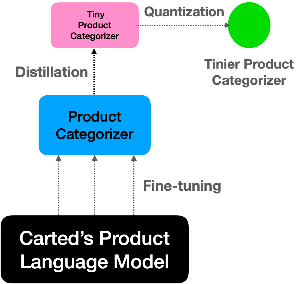
Building a custom, fine-tuned language model

We started by training a (masked) language model on our internal dataset consisting of product titles and descriptions, using a custom variant of RoBERTa.

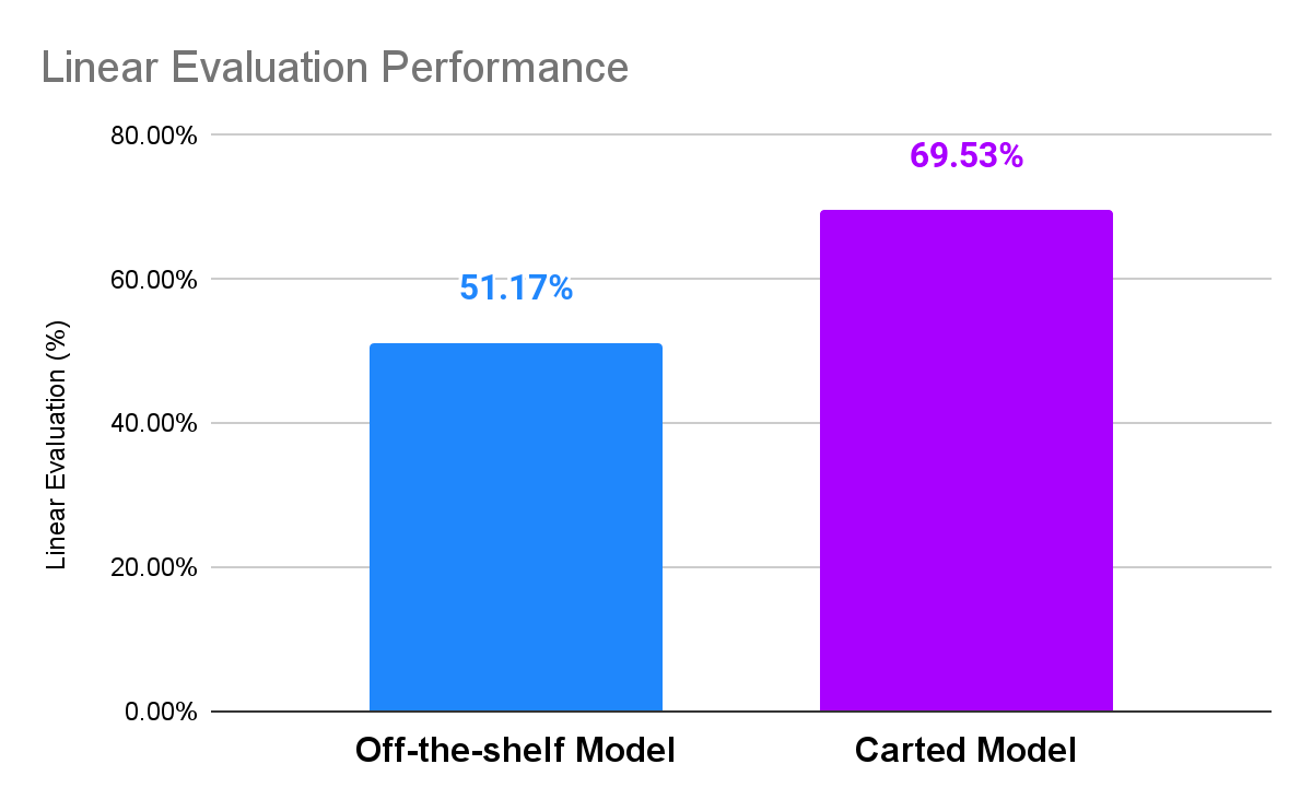
Compared to equal capacity off-the-shelf models, our language model provided significant performance benefits on downstream tasks like product categorization. Having an in-house language model also meant that it could be used for other relevant downstream tasks like product attribute extraction, search relevance, and more. Figure 2 compares the performance of our in-house model to an off-the-shelf equivalent.

We then fine-tuned the language model on our internal product categorization dataset to obtain the initial version of the categorization model. The resulting model provided a top-1 accuracy of 89% on our held-out test set, which satisfied our goal of 85-90% accuracy.

Converting to ONNX for ‘free’ performance gains

ONNX is a model format that provides speed benefits on x86 CPUs without degrading the model’s predictive performance. Since our deployment infrastructure is CPU-based, optimizing the initial version of the model with ONNX was a no-brainer.

With a vanilla ONNX export, we were able to reduce the latency by nearly 40% with very minimal effort. Figure 3 summarizes the gains obtained from the ONNX-optimized version of the original model.

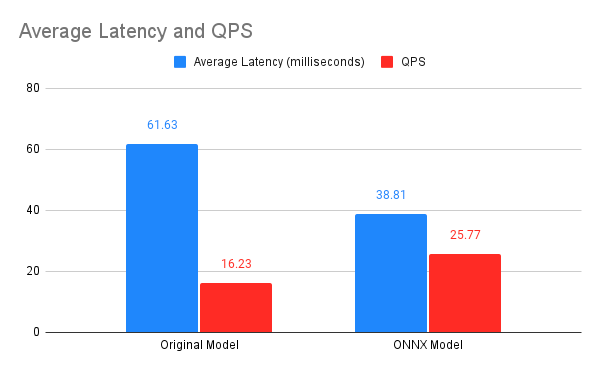
We performed the above benchmark on a c2-standard-8 machine type to leverage its compute-optimized hardware (more on this later). After performing a couple of warm up runs, we reported the final latency and throughput — queries per second (QPS) — averaged across 100 iterations. Lower latency and higher throughput were achieved with the ONNX model.

The benchmark results shown were calculated using a batch size of 1 and a sequence length of 64, however we observed similar behavior across different sequence lengths and batch sizes.

But can we do better? Or more precisely, can we improve the latency further without hurting the predictive performance of the model?

Read on to learn how we experimented to find the answer!

Need for speed

As mentioned earlier, our goal was not only to build an accurate model. Success was also defined as an efficient model that could be cost-effectively deployed to production, and meet the latency expectations of our wider engineering team.

Quantization, pruning, and distillation were the three techniques we examined to optimize the latency of our original model. A summary of our process and findings are described below.

Quantization

In the context of Deep Learning, quantization reduces the numerical precision (for example, from Float32 to Int8) of the parameters and activations. The benefits of this are two-fold:

1. Reduced storage requirements due to the reduced numerical precision
2. Lower latency through faster matrix multiplication

We performed dynamic-range quantization on the original model, which produced a surprising result. Even though quantization is known to have some impact on a model’s predictive performance, in our case, it rendered our model to be about as accurate as a random choice!

Upon further exploration we discovered the root cause of the issue. Our original model uses the SwiGLU activation function since it has shown performance benefits for Transformer-based models. We found out that models using SwiGLU incur a tremendous amount of quantization error.

In Figure 4, we present the histograms of the quantized parameter magnitudes of a Transformer block.

We see that in the SwiGLU chart, the parameter magnitudes are highly-discretized. This makes it difficult to map the quantized values back to their floating-point counterparts during inference. We hypothesized that the quantized version of our original model wasn’t performing well because of this phenomenon.

We incorporated this observation into the rest of the experiments we carried out.

Pruning

During training, a model usually has many weights which can be safely “removed” without incurring much change in the training loss by setting the value of a given weight to zero. In practice, it has been seen that up to 90% of all the weights of a neural network can be removed without any change in the model’s predictive prowess.

This dramatic reduction of the model weights allows for effective compression of pruned neural networks. The secondary advantage is that less compute is required to make an inference as most of the weights are zeros. To do this, the neural network can be re-written such that only the computations involving the non-zero weights are performed, and the rest ignored.

We pruned our trained model and ran our benchmark suite to test for improvements. While there were gains observed thanks to pruning, the gains were limited to the batched setting with a fixed (and large) sequence length, and performance actually regressed for ‘real-world’ scenarios of varying and much shorter product titles. Further details of this experiment are summarized below:

• We started from the original pruned model and then performed Gradual Magnitude Pruning with a target of 75% sparsity using the sparseml package by Neural Magic.
• During training, only the dense matrices of the RoBERTa encoder were pruned.
• The pruned model was converted to the ONNX format and then deployed in the deepsparse engine by Neural Magic.
• The pruned model had an accuracy of 87.9%.
• At a maximum sequence length of 512, the pruned model was 2x faster than the original model.
• In practice, the sequence lengths of the product titles are much shorter, for which the original ONNX model works faster than the pruned model on the deepsparse engine.

Distillation

After the poor results from pruning, we turned to knowledge distillation which distills the so-called ‘dark knowledge’ of a bigger teacher model into a smaller student model. We used the following guiding principles to develop the student model architecture:

• No use of SwiGLU to avoid high quantization errors.
• Parameter initialization from the teacher model following DistilBERT.
• Same model family as followed in FastFormers.

For performing knowledge distillation, we created a custom class inheriting from the Trainer class following the code from this notebook. The student model was a standard RoBERTa with three encoder layers.

Our student model built within these constraints incurred just over a 1% loss in the top-1 accuracy, but it also provided the best performance-speed trade-off. We did not experiment exhaustively with the distillation hyperparameters (such as distillation alpha and temperature). We believe with more hyperparameter tuning, we could have further optimized the accuracy performance.

After obtaining the distilled model, we quantized it using dynamic-range quantization as we did earlier. Somewhat unsurprisingly (due to the removal of SwiGLU), the quantized student model (the distilled model) didn’t incur any drop in predictive performance.

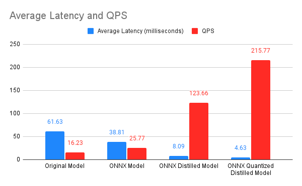
As shown in Figure 5, the quantized and distilled ONNX model brought a significant latency boost — we’re now down to 4.63ms from 61.63ms! The combination of distillation and quantization also resulted in a dramatic size reduction, with the quantized student model weighing in at only 28MBs compared to 466MBs of the original model.

Deployment on Kubernetes with FastAPI and GKE

In this section we walk through our deployment setup and take a look at how the deployed endpoint performed under a simulated production load. In short, we containerized the final (distilled and quantized) ONNX model as a Docker image and deployed it on a Kubernetes cluster. For inference we continued using CPUs, specifically 3rd Generation Intel® Xeon® Scalable CPUs.

Setup

The model was deployed as a RESTful service with the help of FastAPI running on a Kubernetes cluster. The following choices were made to suit our use case:

• The Docker image was constructed by adding layers on top of the python:3.8 image.
• A worker manager such as gunicorn was not used since we wanted the Kubernetes load balancer to manage the pods. For the same reason, we served the model using a single uvicorn worker.
• We configured the horizontal pod autoscaling (HPA) to trigger if CPU utilization reached 60%. This was specific to the load testing setup we used. A higher percentage led to stalling during testing, and was not an issue we needed to triage at this time.
• We found that configuring CPU requests and CPU limits is unnecessary as the ONNX model is designed to use all the CPUs in parallel to maximize throughput.

Infrastructure

• We automated the provisioning and the de-provisioning of the Google Cloud Platform (GCP) VMs using Terraform.
• kustomize and kubectl are used to deploy our FastAPI image to the VMs provisioned by Terraform.
• To benefit from the parallel processing abilities of the ONNX runtime, we needed to use a VM with a CPU supporting AVX 512 instructions. We decided upon the c2 (or compute-optimized) instances offered by GCP, which offer the 3.9GHz Intel Cascade Lake processors. Specifically, we used the c2-standard-8 instances, where the 8 stands for the number of CPUs.

Load testing

One of our goals was to deliver an endpoint that can withstand a large volume of requests per second. To simulate this and monitor how the system performs under the stress, we decided to use Locust, an open-source Python-based load testing tool. Our load-testing setup was heavily inspired from the workflow presented in this article. We took the following steps to configure Locust and perform load testing:

• A master pod with 1 replica to control the Locust workers.
• 5 replicas of the worker pod that would perform the actual load tests.
• We used a separate VM to port-forward the master pod’s port to our local machine via SSH to run the load test via the browser.
• In total, we spawned 2000 workers with 5 workers being spawned per second.
• We deployed the API with HPA set to spin up a maximum of 3 replicas for the sake of load testing.

After running the load test, we observed that the system did not fail for a single request, although average latency increased rapidly as the number of requests per second increased.

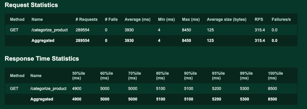
As shown in Figure 6, latency during the test was as low as 4ms. The max and average latencies are very high, but it’s important to consider that these latencies are computed under high load and will not reflect usual working conditions.

Conclusion

In this post, we shared our journey of obtaining a high-accuracy, low-latency product categorization endpoint, including a look at how the endpoint would perform in production with simulated load testing. We hope the approaches discussed in this post will help make your model endpoints faster and cheaper to run!

Acknowledgements

Utilizing tools provided by Hugging Face made our workflows more productive and enjoyable. We leveraged transformers to build our models and perform data preprocessing, datasets to manage our training data, evaluate to compare the different variants of the models we tried out, and Hugging Face Hub to manage all of the artifacts.

Their tools let us focus on the core parts of our business while delegating away the boilerplate code. We recommend taking a look at their excellent resources for your own projects.